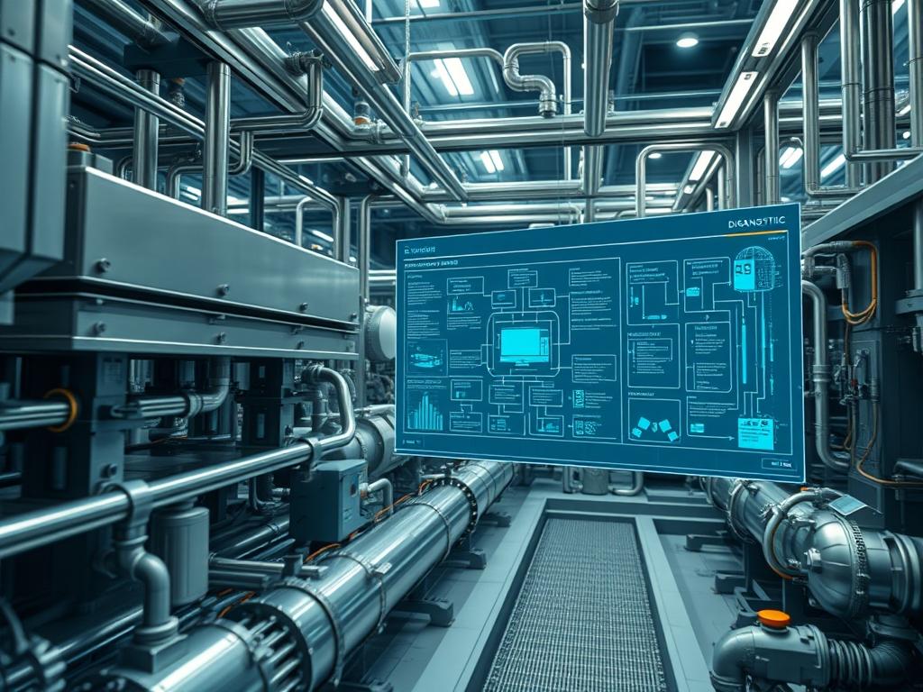
Desalination ROI Modeling serves as the foundational decision-support framework for municipal infrastructure, bridging the gap between high-pressure fluid dynamics and econometric forecasting. As water scarcity accelerates due to shifting climatic patterns; municipalities must transition from reactive procurement to predictive financial engineering. This model provides an idempotent approach to assessing the Levelized Cost of Water (LCOW) by integrating real-time energy prices, membrane degradation rates, and debt-servicing schedules. Within the technical stack, the ROI model functions as the analytical layer sitting atop the Supervisory Control and Data Acquisition (SCADA) system and the Enterprise Resource Planning (ERP) suite. It resolves the problem of volatile operational overhead by simulating various energy-mix scenarios and thermodynamic efficiencies. By establishing a rigorous baseline for capital deployment; the model ensures that the substantial energy payload required for Reverse Osmosis (RO) is offset by long-term resource reliability and reduced reliance on external water imports.
Technical Specifications
| Requirement | Default Operating Range | Protocol/Standard | Impact Level | Recommended Resources |
| :— | :— | :— | :— | :— |
| Feed Water TDS | 35,000 to 45,000 mg/L | ASTM D4194 | 10 | High-Salinity Sensors |
| Energy Recovery Efficiency | 92% to 98% | ISO 50001 | 9 | Isobaric Chambers |
| Membrane Permeate Flux | 12 to 18 GFD | NSF/ANSI 61 | 8 | 8-inch Spiral Wound |
| System Concurrency | 50 to 500 Simulation Threads | IEEE 1012 | 7 | 8-Core CPU / 32GB RAM |
| API Latency | < 150ms | REST/JSON over HTTPS | 5 | 1Gbps Fiber Uplink |
| Data Logging Interval | 1s to 60s | Modbus/TCP | 6 | 1TB NVMe Storage |
The Configuration Protocol
Environment Prerequisites:
Before initializing the ROI modeling environment; the lead architect must verify that all data ingestion pipelines are compliant with IEEE standards for power quality and ISA-95 standards for enterprise-control system integration. The modeling engine requires Python 3.10 or higher with the following libraries: numpy, scipy, and pandas. On the hardware side; ensure the Reverse Osmosis (RO) skids are calibrated to transmit high-resolution pressure and flow data via the port 502 Modbus interface. Administrative access to the municipal cloud environment is mandatory; specifically, the user must have sudo privileges on the local analytics gateway and read-only access to the SCADA historian database.
Section A: Implementation Logic:
The engineering design of a Desalination ROI Model relies on the encapsulation of thermodynamic variables into a financial logic gate. The primary objective is to minimize the energy-per-cubic-meter ratio while maximizing the recovery rate. This is achieved through a multi-stage simulation that accounts for signal-attenuation in sensor arrays and thermal-inertia in the high-pressure pumping system. By modeling the pump-membrane interface as a series of constant-pressure nodes; the architect can predict precisely when the cost of increased energy consumption (due to membrane fouling) exceeds the cost of a scheduled maintenance shutdown. This predictive maintenance scheduling is the core driver of ROI; it prevents packet-loss of operational data and ensures the long-term throughput of the permeate stream.
Step-By-Step Execution
1. Initialize the Financial Modeling Kernel
Deploy the core ROI analytical package by navigating to the project directory and executing python3 -m venv roi_env. Once the environment is activated; install the required econometric packages using the command pip install desal-analytics.
System Note: Initializing the virtual environment isolates the ROI calculation logic from the system-wide library versions; preventing dependency conflicts between the water-ops scripts and general municipal software.
2. Configure SCADA Data Ingestion via Modbus
Modify the configuration file located at /etc/desal/modbus_bridge.conf to point to the IP addresses of the PLC (Programmable Logic Controller) stack. Ensure the polling frequency is set to a 5-second interval to capture transient pressure spikes that impact energy volatility.
System Note: This action establishes a high-performance socket connection to the physical asset; defining the throughput of raw physics data into the financial simulation layer.
3. Calibrate Energy Recovery Device (ERD) Metrics
Execute the calibration script ./calibrate_erd.sh –target-efficiency 0.96. This script queries the current isobaric chamber performance and inputs the values into the ROI variable ERD_Effic.
System Note: High-efficiency energy recovery significantly reduces the kilowatt-hour (kWh) cost of permeate; this step directly modifies the overhead variable in the LCOW equation.
4. Establish Secure Database Connectivity
Update the database connection string in ~/config/db_secrets.json with the credentials for the encrypted PostgreSQL instance. Use the command chmod 600 ~/config/db_secrets.json to restrict access to this file.
System Note: Restricting file permissions prevents local users from accessing sensitive financial metadata; hardening the ROI model against internal unauthorized modifications.
5. Run the Monte Carlo Sensitivity Simulation
Trigger the primary ROI engine using roi_engine –run-sim –iterations 10000 –output ./reports/q4_forecast.pdf. This will process the historical energy price volatility and membrane lifespan data to generate a probability distribution of the ROI timeline.
System Note: The high concurrency of this operation stresses the CPU; the systemctl process manager may be used to prioritize this task via systemctl set-property roi_engine.service CPUWeight=200.
6. Verify Log Integrity and Output
Check the system journal for any errors during the simulation by running journalctl -u roi_engine -f. Search for any instances of “NaN” or “Infinity” in the numerical output which may indicate a division-by-zero error in the osmotic pressure calculation.
System Note: Continuous log monitoring identifies sensor signal-attenuation or physical fault codes that could poison the financial dataset with inaccurate telemetry.
Section B: Dependency Fault-Lines:
The most common point of failure in Desalination ROI Modeling is the misalignment between physical equipment upgrades and the software-side depreciation schedule. If the RO membrane manufacturer is changed without updating the membrane_rejection_rate variable in the config file; the resulting ROI projections will be invalid. Furthermore; latency in the SCADA-to-Cloud bridge can result in outdated energy pricing data being used for the LCOW calculation. Another critical bottleneck is the thermal-inertia of the intake water; as seasonal temperature changes affect membrane permeability; the model must dynamically update its flux-correction factors to maintain accuracy.
THE TROUBLESHOOTING MATRIX
Section C: Logs & Debugging:
When the model produces anomalous ROI results; the first point of inspection is the log file located at /var/log/desal_roi/engine.log. Look for error code ERR_SCADA_TIMEOUT; this indicates that the analytics engine cannot reach the physical sensors; likely due to a firewall rule blocking port 502 or port 443. If the simulation results show a sudden drop in ROI; check the sensor readouts for Feed_Conductivity_High; this suggests a breach in the intake filtration system which will drastically increase the chemical dosing overhead.
Path-specific debugging involves checking /opt/roi_model/lib/python3.10/site-packages/ to ensure that no conflicting versions of the scipy library have been installed. A mismatch here will cause the solver to fail during the non-linear optimization of the energy-curve. If physical fault codes like E004 (High Delta-P) appear on the pump controllers; the ROI model should be manually paused using systemctl stop roi_engine to prevent the ingestion of outlier data during mechanical stress tests.
OPTIMIZATION & HARDENING
– Performance Tuning: To increase simulation throughput; the architect should leverage the multiprocessing module in Python to spread the Monte Carlo workload across all available CPU cores. Tuning the kernel’s virtual memory management via sysctl -w vm.swappiness=10 reduces I/O wait times during large-scale data ingestion.
– Security Hardening: All telemetry data must be encapsulated via TLS 1.3 during transit. Use iptables to restrict incoming traffic to the SCADA gateway to only known IP addresses of the municipal operations center. Set up a physical fail-safe logic in the PLC that overrides any software commands from the ROI model if pressure exceeds 1050 PSI.
– Scaling Logic: As the municipality adds more desalination trains; the model should scale horizontally. Use a Dockerized container approach for the ROI engine; allowing new instances to spin up for each new RO skid. Use a load balancer to manage the API requests to the ROI dashboard; ensuring no single node becomes a bottleneck for financial reporting.
THE ADMIN DESK
How do I adjust for sudden energy price spikes?
Modify the energy_volatility_buffer in the /etc/desal/parameters.json file. This increases the margin of error in the ROI calculation; ensuring that the municipality remains budget-positive even during periods of extreme energy market instability or peak-load pricing.
Why is the model overestimating membrane life?
Check the fouling_index_coefficient. If the physical pre-treatment system is underperforming; the real-world membrane degradation will outpace the theoretical model. Update the coefficient based on the latest SDI (Silt Density Index) tests performed at the intake site.
Can I run this on-premise without cloud access?
Yes. Use the –local-mode flag when starting the service. This redirects all API calls to a local SQLite database and bypasses the cloud-based forecasting module. Ensure you have sufficient local storage to handle the increased time-series data payload.
What is the “Critical Capex Divergence” error?
This error occurs when the projected maintenance costs exceed the initial budget by more than 20%. Verify the inflation_adjustment_rate in the configuration. It often triggers if the local currency has devalued significantly against the procurement currency for RO parts.
How is signal-attenuation handled in the telemetry?
The model employs a Kalman filter to smooth out noise from the pressure sensors. If the noise floor exceeds the threshold; the system triggers a warning in the journalctl logs and uses the last-known-good-value for the LCOW calculation.